Hyperspherical Variational Auto-Encoders

“OMG, have you seen [insert latest OpenAI GPT model], isn’t it amazing !???”

For all those who are getting a little irritated at the sheer quantity of noise in the recent hype cycle, and of all the former web3.0/crypto-heads now going “all-in” on AI: you’ve come to the right place. Let’s forget about the hype and about how we’re all supposedly going to die, heck let’s even forget about the transformer architecture and GPT-style generative models. Instead, why don’t we lay back, do some math, and have a look at another type of probabilistic generative model - the variational autoencoder (VAE). Don’t worry, this won’t be the million-th blog post explaining how these work, instead I’ll be diving into a recent(ish) flavor of VAE: the Hyperspherical VAE. These modify the posterior to use non-Gaussians distributions such as the von Mises-Fisher (vMF) distributions, which can be interesting when we expect the latent structure to exhibit some hyperspherical properties. Plus, not only does hyperspherical latent structure sound cool but it also gives some neat visualizations. So, if you have 5 mins of your precious time to spare, we can go through the paper together and I’ll show you a few fun experiments we were able to implement which allowed us to play with the original code and try to bump performance a little.

A primer on VAEs

If you’re still reading at this point, I’m guessing you weren’t bored by the ML jargon above and hopefully this means you also already kind of know how a VAE works. For our purposes, a VAE looks something like this:

You take input data \(X \in \mathbb{R}^{n \times d}\) (\(n\) samples and \(d\) dimensions) which you represent by a latent variable \(Z\). Now, in a traditional autoencoder, \(Z \in \mathbb{R}^{n \times d_{latent}}\) will usually be the output of a neural network that simply has an output dimension \(d_{latent}\) which is smaller than \(d\). You compress the data to a latent space with fewer dimensions, then de-compress it using a neural network decoder back into the original space. The variational framework changes this by considering probabilistic representations for \(X\) and \(Z\). This means each input will be encoded into a distribution rather than a single value. You may be wondering at this point, why is using probabilities interesting and why should we care about having a latent distributional encoding?

Well, if we consider \(X\) to follow a certain distribution, we can frame the problem as maximizing the log-likelihood of the data \(\log p_{\tau}(x)\) where \(\tau\) parametrizes our input data distribution. This is interesting as if we have the “optimal” parameter that adequately describes our input distribution, then we can sample from the input space directly which means generating new images (hence the name probabilistic generative model). Since the images will be drawn from the “same” distribution as our training set, hopefully this means these won’t look like random noise. The problem is that we don’t know how to optimize \(p_{\tau}(x)\) directly. Let’s imagine an input space of images of cats, you can’t really say “let’s find the best mean and stdev for a multi dimensional gaussian that fits these images” - no gaussian distribution would ever fit that remotely well. Instead, we can consider a latent variable \(Z\) that generates our observations. The nice thing is, we can imagine this latent variable to follow any distribution we would like. This means if we can reframe the optimization of our likelihood to include terms with respect to our latent variable, we have a fighting chance of being able to include reasonable prior assumptions and actually compute the thing.

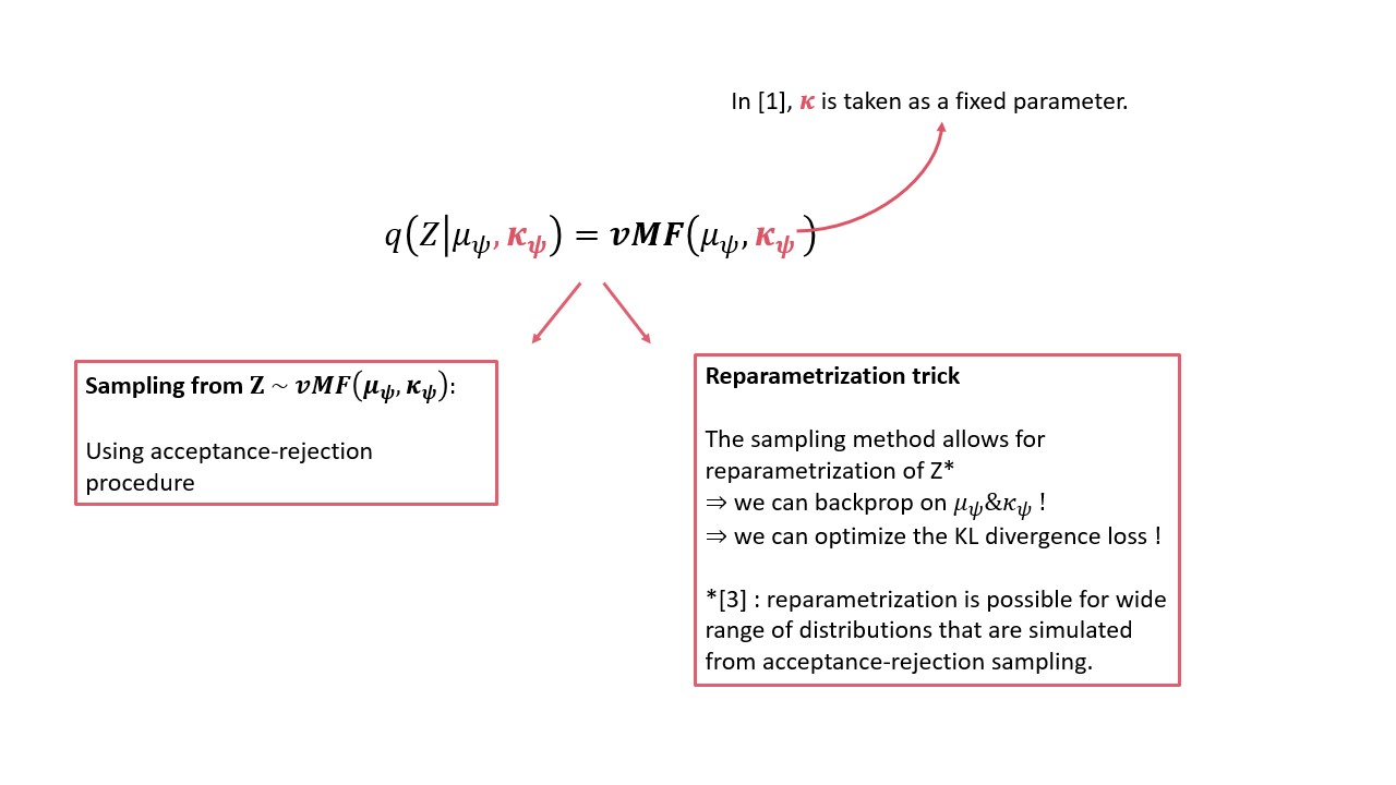
More mathematically, consider \(\log p_{\tau}(x)\) within the variational framework: we marginalize over the latent space distribution \(p_{\tau}(x) = \int_{z}^{} p_{\tau}(x, z) \,dz\) and rewrite this is as \(p_{\tau}(x) = \int_{z}^{} p_{\tau}(x \| z)p_{\tau}(z) \,dz\). Without going into further detail (see Wiki), you can optimize a lower bound of the log of this integral by maximizing the Evidence Lower Bound (ELBO) \(\mathbb{E}_{q_{\psi}(z \| x)}[ \log p_{\theta}(x \| z)] - KL(q_{\psi}(z \| x) \| p_{\tau}(z))\). Here, \(q_{\psi}(z \| x)\) represents our approximate posterior distribution (which is why we use q and not p). This approximate posterior is taken from a family of distributions (e.g. gaussian or vMF as we will see later) and we parametrize it by \(\psi\). In practice this parametrization refers to the encoder neural network that will output the parameters of the posterior distribution given an input. In the simplified VAE shown above, these parameters correspond to the mean and standard deviation of a gaussian distribution. The main idea of the paper is to consider a vMF distribution for the posterior which gives the latent space “hyperspherical” properties. They also provide the theoretical work needed to backpropagate to find the parameters of the vMF distribution where previous work had considered one of the parameters as constant.

The vMF distribution

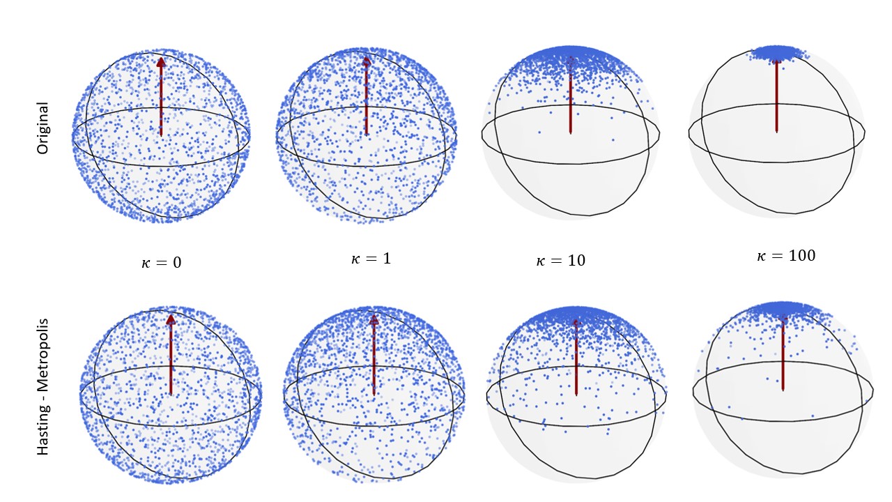
The von-Mises Fisher distribution is interesting to consider as a prior for a number of reasons. First, it is not a gaussian. This may sound kind of dumb but honestly, it is not a bad first-order approximation to say that sometimes the best you can do to try and improve a certain method is to find where the algorithm relies on the assumption that the underlying distribution is gaussian and ditch that. A little more seriously, the von-Mises Fisher is adapted for hyperspherical distributions. Specifically, it is a probability distribution defined on the surface of a hypersphere (a sphere in a potentially high-dimensional space). As you can see in the cute visualization below, it’s quite useful to model directional data on this hypersphere as the \(\kappa\) parameter controls the concentration of the distribution around a specific direction. The pdf looks like this \(f(x \| \mu, \kappa) = C(\kappa)\exp(\kappa \mu^T x)\) where \(x\) can be of any dimension. For our purposes we don’t really need to know what \(C(\kappa)\) is (it’s just a normalization constant) but what’s import to note is that as \(\kappa\) increases, the distribution gets more concentrated around the mean \(\mu\) direction.

Some messy code shows this very well:

KL divergence and vMF sampling

Since everything is probabilistic, to decode an input with the decoder we need to be able to sample from the latent space. Also, to backprogate the loss and update the distribution parameters (all the guides I was mentioning should have explained to you how the reparametrization trick helps with this) we need the reparametrization trick to make sure we can actually differentiate with respect to the distribution parameters. The paper deals with both of these issues nicely. The main component of the vMF sampling corresponds to acceptance rejection sampling with a clever reparametrization trick you can see highlighted below:

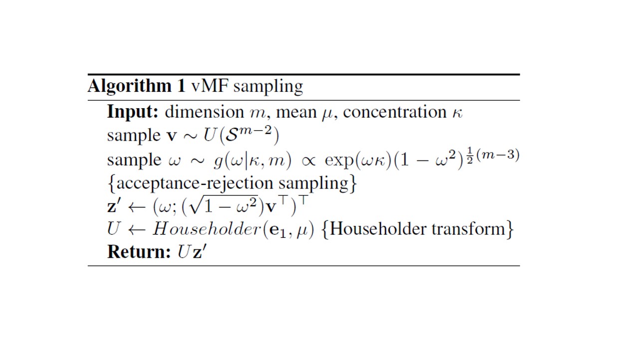
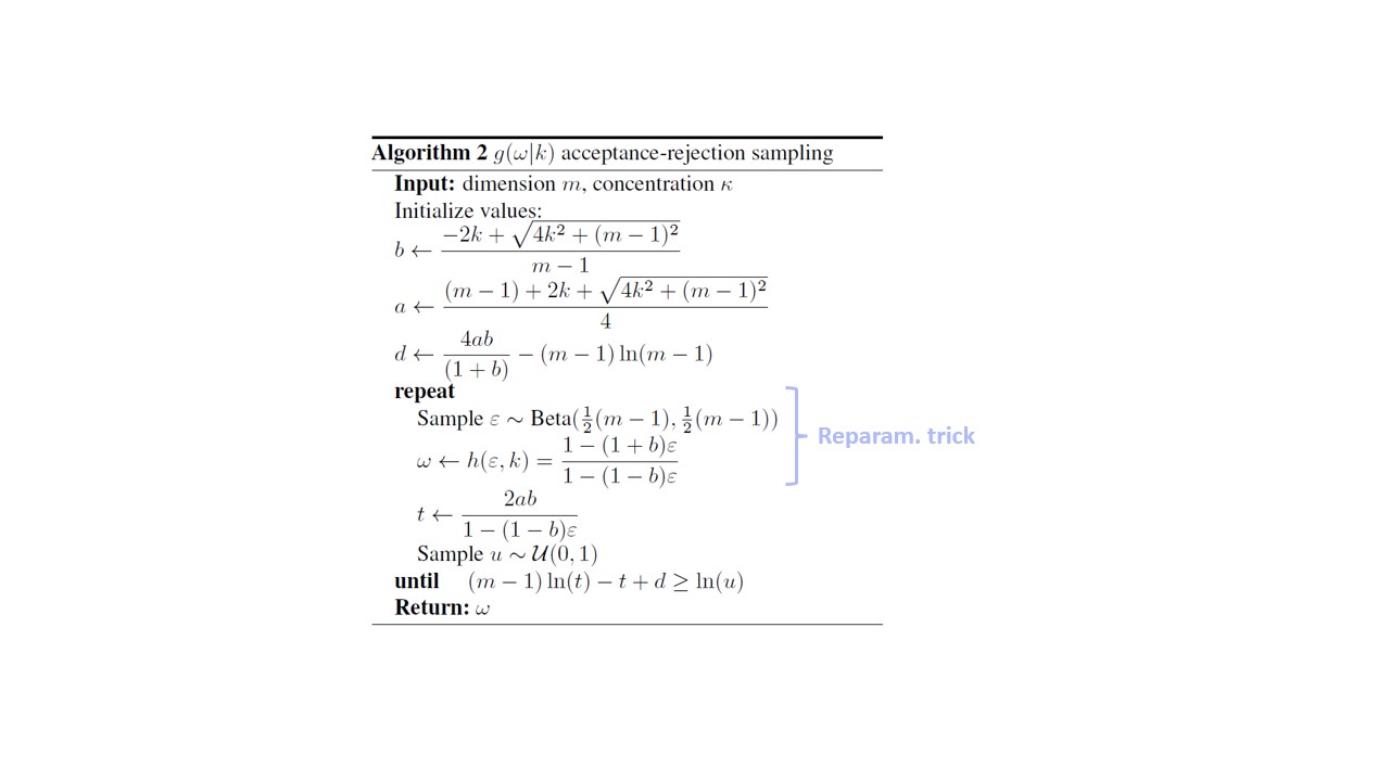
Although the specifics are somewhat painful, we sought to see if we could play around with the sampling implemented in the paper. Was there perhaps a better sampling method? Would it impact performance?

Modifying the sampling mechanism from the original paper

So, we looked into how we could modify the acceptance rejection sampling to something else. This was really more to get a sense of the code and to implement a sampler rather than because some theoretical insights might have suggested a better sampler could improve the H-VAEs performance. You can see below the exact sampling algorithm we decided to implement (the Metropolis-Hastings algorithm) which basically amounts to just changing the ratio used to reject samples.

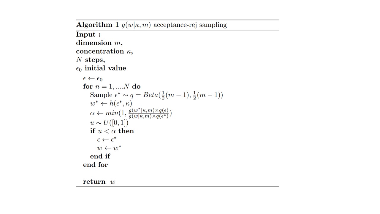
It was fun to be able to code this and to see if there was any real impact on performance/how the samplers differed. We can actually compare the new sampling without all the VAE around it. Let’s take the sampling of the vMF we saw previously and compare it to the HM sampler. We can see that the HM is slightly more exploratory with a distribution that seems to be more spread out for a same value of \(\kappa\).

MNIST reconstruction

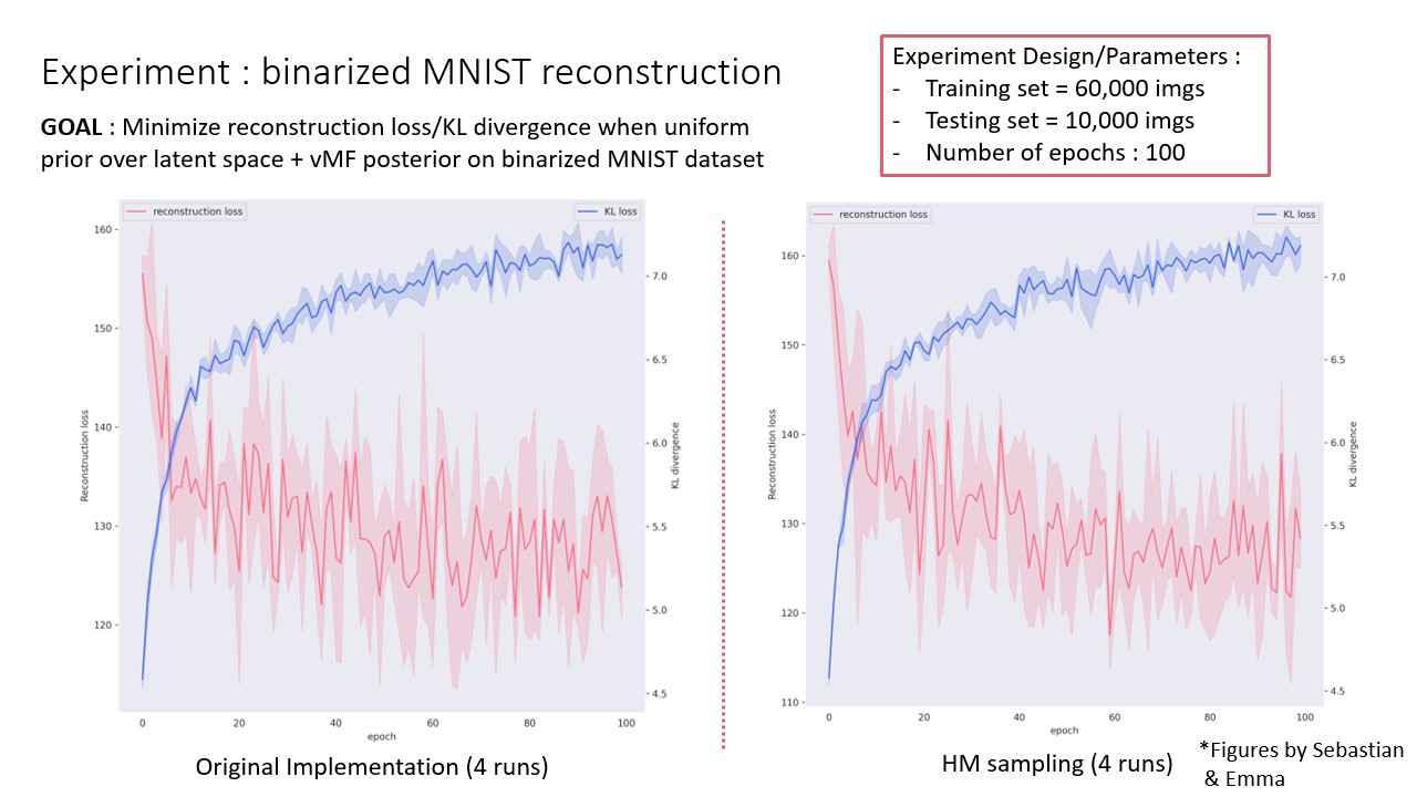
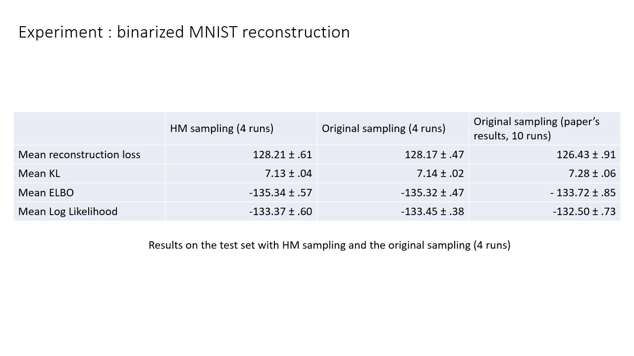
(Yes, we’re still using MNIST for experiments, even in 2023…). The final thing we wanted to test was to see if this modified sampling actually had any impact on this H-VAEs performance. To test this, we take the one and only OG MNIST dataset. The experiment solely consists in running the training of the H-VAE on MNIST and then looking at the training and testing performance when we use either sampler. Long story short, there’s no real training or testing loss performance. This was kind of to be expected since we did not change the sampler substantially but, intuitively, if you’re able to sample better from the posterior distribution your performance shoult get better.

Visualizing the latent space

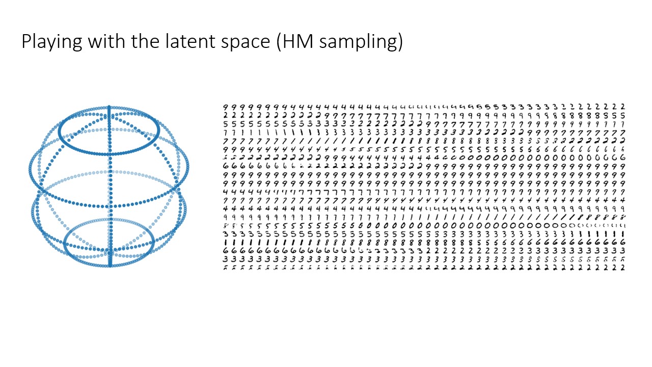
Finally, for some cool visuals, it’s always nice to look at the latent space. In this case, we can look at how the various MNIST digits are distributed across the hypersphere and how digits that resemble each other lie closer in the latent space.