Graph Transformers

You can find all the code here and the original report Emma Bou Hanna & I wrote here.

Abstract

The goal of this project is to study how transformer networks can be adapted to work on graphs. As transformers have shown impressive performance in various domains (NLP, computer vision), some have tried to adapt the architecture to solve learning problems on graphs. Mainly focused on recent work (Dwivedi & Bresson, 2020), our report will provide a critical perspective highlighting the main strengths and limitations of such methods.

Introduction

Relevance

Graphs permeate most areas of modern-day science. Indeed, these seemingly abstract mathematical objects and data structures are used in virtually every scientific field with some underlying non-Euclidean space: chemistry (computational modelling of molecules), computer science (communication networks, computation graphs), linguistics (semantic networks), biology (protein networks, transcriptional regulation, …) and high-energy physics. Given the relevance and ubiquity of graphs, a few categories of important problems can be distinguished. The first category are the natural learning problems that arise where predictions can be made by using graph-structured data as features. These prediction problems can be further broken down into graph feature-level (nodes, edges) problems and graph-wise problems. Recommending friends to a user on social media is one example of an edge prediction problem, identifying a bot is an instance of a node classification problem and predicting the chemical properties of a molecule based off its structure is a graph wise problem. What unites these previous problems is really the prediction aspect, the learning of an analyzing function defined on the non-Euclidean space of graphs. Another very important class of problems is graph representation learning (Hamilton et al., 2017), i.e how to efficiently and accurately encode a graph into a low-dimensional embedding such that the graph’s structural information is integrated into the embedding. This problem class overlaps with the previous but they do form disjoint sets. In many cases, efficiently encoding a graph into a low dimensional latent space makes the downstream tasks of classification or regression much easier and can be optimized for jointly with the desired task. In these cases, learning a good latent space goes hand-in-hand with making good predictions clearly showing how the two main problem classes overlap. In other cases, one may seek to perform this encoding in an unsupervised manor without any downstream prediction task playing on the optimization of the embedding. To put it into context, the work mainly studied here fits into this intersection of being both a representation learning problem and a prediction problem as the transformer architecture encodes the graph’s information before a downstream network is able to perform any actual prediction task.

Related work

Both graph representation learning and prediction problems have improved at a rapid pace over the past decades. Traditional approaches in graph representation learning first relied on extracting summary graph statistics (Bhagat et al., 2011), and features or using kernel functions (Vishwanathan et al., 2008). Kernel methods use kernel functions as a measure of similarity between objects of the input space. On graphs, these kernels can take many forms and can operate on elements of the graph or the graphs themselves. However, although some of these methods have been shown to be computationally efficient, pre-engineered features or pre-picked kernel functions have very strong inductive bias and are inflexible. Much like in non-graph machine-learning, the ability to learn encoded representations rather than extracting features by hand has become a sought after property of modern algorithms. These algorithms learning encoded representations vary from factorization-based approaches using laplacian eigenmaps (Belkin & Niyogi, 2001) to random-walk based approaches such as node2vec (Grover & Leskovec, 2016) and finally deep-learning based methods (Scarselli et al., 2009) one of the most recent ones being the main work focused on here (Dwivedi & Bresson, 2020).

Problem definition

We define a graph as a set of nodes and edges \(G = (V, E)\), with \(E \subseteq \{ (x, y) | (x, y) \in V^2, x\neq y \}\). We first consider homogeneous weighted (single type of node and edge) graphs (at this point, no distinction is made between directed/undirected). Each node \(i\) is characterized using a vector \(x_i \in \mathbb{R}^{d_f}\), \(d_f\in\mathbb{N}^*\) being the number of features, and a discrete or continuous label \(y_i\). For a graph with \(|V| = N\) nodes, we denote \(X \in \mathbb{R}^{N \times d}\) the node feature matrix, \(y \in \mathcal{Y}\) the node labels, \(A \in \mathbb{R}^{N \times N}\) the adjacency matrix, where \(A_{ij} = 1\) if \((i, j)\) or \((j, i) \in E\) and \(0\) if not and \((\beta_{ij})_{i, j \in [\![1, N]\!]} \in \mathbb{R}^{d_e}\), \(d_e\in\mathbb{N}^*\) the edge features. We consider two main types of graph learning problems in this report: node classification (an instance of node-wise problems) and graph regression (an instance of graph-wise problems).
Given \(X\), \(A\) and \(\beta_{i, j}\), node classification with m discrete classes consists of predicting \(y \in \{0, 1\}^{N \times m}\), the one-hot encoding of our node labels. Graph regression, on the other hand, aims at predicting a single scalar value \(y \in \mathbb{R}\).
To solve these two learning problems (amongst others), geometric deep learning (Bronstein et al., 2017) aims to use deep neural networks to learn the mapping, which we call \(f_{\theta}\), between input and target spaces. As has been mentioned previously, in many cases \(f_{\theta}\) can be decomposed as \(f_{\theta} = f_{pred} \circ f_{enc}\) the composition of two functions: the encoder (representation learning) and prediction function. Graph neural networks (GNNs) (Scarselli et al., 2009) have obtained impressive results on these tasks but the wide success of transformer-based models in NLP begs the question as to whether these might be able to perform even better. Indeed, natural language can be viewed as a subclass of fully-connected graphs where each word represents a node. So if transformers efficiently and accurately learn \(f_{\theta}\) when the input space is a constrained form of graph, is it possible to modify the architecture to maintain performance when we generalize the input space?

Proposed solution

In (Dwivedi & Bresson, 2020), the authors adapt the transformer structure to more generic homogeneous graphs than what can be found in NLP. These graphs are not necessarily fully connected like tokens (generalized words) in a sentence would be, and the authors claim that their model is abstract enough to deal with this larger problem class.

Transformers

Traditional transformers have two main inputs, that need to be clearly defined when dealing with arbitrary graphs. In the context of NLP, the authors of the original paper (Vaswani et al., 2017) define an embedding, which we denote \(E^k\), and a positional encoding \(P^k\) for each token \(k\). A sinusoidal encoding of the position is often used for the latter.

Positional encodings are the best way of making use of the sequence order, in the absence of convolutions and recurrence. They should ideally be deterministic encodings, unique, and distance between any two words should be consistent across sentences with different lengths. In (Vaswani et al., 2017), the authors introduced a sinusoidal positional encoding :

where \(k\) is the kth word and \(i\) is the ith dimension. This sinusoidal encoding essentially replaces the index of a token in a sentence (k in this case) so that it stays in normalized range and is able to deal with variable length sequences. Mapping each index to a vector whose components are defined above also means that the positional encoding can be added to the embedded representation through a simple term by term addition, making it all the more computationally efficient while still uniquely including positional information.

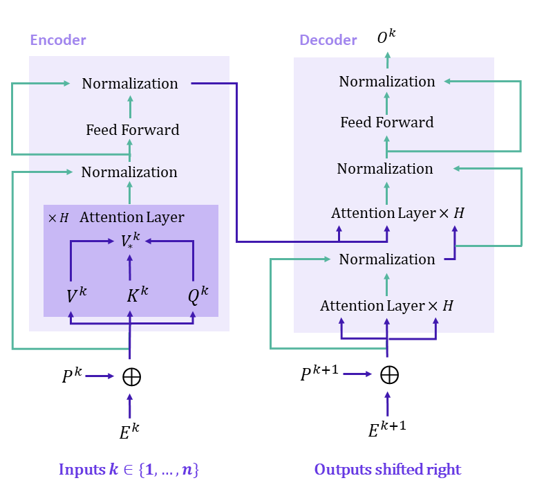
The network then outputs a prediction based on a characterization of each word as well as its position in the sentence. This can be achieved by summing \(P^k\) and \(E^k\), which have the same dimension. Relations between all words are then determined through an Attention Mechanism, which highlights the influence that all words have on each other by computing dot products between embedded feature vectors. More specifically, we compute a query embedding \(Q^k\) for each word as well as key \(K^k\) and value \(V^k\) embeddings. Both \(Q^k\) and \(K^k\) have dimension \(d_k\). We then compare each word \(k\) with all other words and compute an aggregated value \(V_*^k\) that takes into account the influence of all other words. Mathematically : \(V_*^k = softmax(\frac{Q^k K^T}{\sqrt{d_k}})V\) This value will then serve as an enhanced embedding of the word \(k\).

This translates in the network represented in Figure 1 where we stack attention layers before normalizing and using a fully-connected layer. The Attention mechanism can capture long-range dependencies as the dot product is calculated between every input token, however this also means that the complexity is quadratic in the input dimension. This will become problematic as soon as we want to apply the transformer to an input with a larger number of tokens that what we may find in a sentence for NLP.

Graph Transformers

To adapt the architecture to graphs, we need to find the relevant inputs \(E^k\) and \(P^k\). The simplest input to choose is \(E^k\), which can be represented by our node features \(X^k\) defined in subsection 1.3.

Positional encodings may be more tricky to find because the goal would be to generalize the sinusoïdal positional encoding of words introduced in the original paper. (Dwivedi & Bresson, 2020) makes the hypothesis, like other papers before them, that Laplacian eigenvectors could be used to provide information of relative localization for each node. Laplacian eigenvectors can be calculated based on the adjacency matrix \(A\) and the degree matrix \(D\) defined as such :\(D_{ii} = Card(\{j|(i,j) \in E \})\) and \(D_{ij} = 0\) for \(j \neq i\). Then, \(L = D - A\) and the factorized laplacian matrix \(\Delta = I - D^{-\frac{1}{2}}AD^{-\frac{1}{2}}\) can be decomposed in an eigenbase of real numbers because it is a symmetric matrix with coefficients in \(\mathbb R\). This means we can effectively compute the Laplacian eigenvectors to use as positional encoders.

Regarding the actual Transformer architecture, the authors chose to keep the same encoder as the one we represented in Figure 1, the main difference with (Vaswani et al., 2017) being how they normalize their \((V_*^k)_{k \in [1, N]}\) (with BatchNormalization here). The main advantage of BatchNormalization is to normalize per feature, which can be really useful when dealing with node features with different scales. No decoder is needed here, as the tasks consist in classification or regression, therefore the authors chose to add MLP layers on top of this encoder to perform these specific tasks.

To truly parse the entirety of the information given by the graph, the edge features \((\beta_{ij})_{i, j \in [\![1, N]\!]} \in \mathbb{R}^{d_e}\) also need to be included in the computation of the encoded representation. In the graph transformer architecture, these edge features intervene in the calculation of \(V_*^k\), thanks to the following operation :

\(V_*^k = softmax(\frac{Q^k K^T}{\sqrt{d_k}}\odot \beta_k)V\) where \(\odot\) denotes the elementwise product. It is natural to make the edge features intervene at this step of the calculation, as the dot product \(Q^k K^T\) calculates the influence of all other nodes on node \(k\), and this influence should be weighted by edges linking nodes to \(k\), hence the elementwise product.

Experiments

The results demonstrate good performance on graph regression problems (ZINC dataset) as well as node classification tasks (CLUSTER + PATTERN datasets). Indeed, the experiments that were conducted by the authors showed relative performance on these different tasks compared to GCN, GAT, GatedGCN. The indicators used to showcase these results are the Mean Average Error (MAE) for graph regression, as well as the accuracy for node classification. It is important to note that Graph Transformers at this stage seems to be more of a Proof of Concept than a truly competitive architecture for graph-related tasks since performance is worse than GatedGCN for every dataset and the number of datasets which were benchmarked is quite limited. The paper analyzed here is clearly an initial building block for later work to improve upon.

Importance of graph sparsity and positional encoding

First, contrary to NLP problems where tokens can be treated as a fully connected graph, real graphs may have an arbitrary number of nodes, which prevents them from being treated as fully connected. For memory management and computation time, it is therefore useful to exploit the graph’s sparsity, where each node relates to its immediate neighbors. An interesting question arises as attention was initially introduced to capture long-range dependencies by comparing all tokens in the attention layer. Here, it is clearly infeasible to do so for graphs with more than a few hundred nodes yet we might wonder how useful the attention mechanism is if we only limit ourselves to the neighborhood of each node, except for arbitrary large neighborhoods. The exploitation of graph sparsity translates explicitly in the calculation of the attention output of each layer (let’s consider only one attention head for simplicity) : \(h_i^{out} \propto \sum_{j \in N_i}V_*^{ij}h_j^{in}\) where \(N_i\) is the neighborhood of the node \(i\), and \(h_i\) the corresponding representation of node \(i\) before (\(h^{in}\))and after (\(h^{out}\)) going through our layer. Sparsity of the graph is also taken into account through the usage of edge features, which can be interpreted in most cases as links strength.

Second, choosing a good positional encoding is vital for the sake of good predictions as we highlighted in Section 2. The authors stress that Laplacian eigenvectors can be viewed as a generalization of sinusoidal positional encodings which make them the perfect candidates. To go further, they perform an in-depth comparison to the positional encodings used in Graph-BERT (Zhang et al., 2020). They perform an ablation analysis by swapping the Laplacian eigenvectors by Weisfeiler Lehman based absolute PE (WL-PE) or no PE whatsoever. WL-PE are obtained by performing \(k\) steps of the Weisfeiler Lehman algorithm, which we will explain in Section 3. The results obtained with both methods on the same datasets allow them to conclude that Laplacian eigenvectors give better performance.

Limitations

This paper presents several limitations, which can be organised into three parts.

Pertinence of Laplacian positional encodings

To justify their choice of Laplacian eigenvectors as good candidates for positional encodings, the authors cite (Dwivedi et al., 2020), which states that these eigenvectors could be a good generalization of traditional positional encoding vectors, because laplacian eigenvectors of fully connected graphs (like in NLP problems) are the cosine and sinusoidal functions. This seems to draw from a parallel with physics, where the Laplacian operator (divergence of the gradient) has eigenfunctions that are sines/cosines. However, we could not find any paper giving a mathematical intuition of this hypothesis or a rigorous explanation as to why this works for the graph laplacian. We therefore decided to mathematically verify this in the case \(N=2\) nodes, linked by an edge.

We can derive the degree matrix \(D\) and the adjacency matrix \(A\) as such :

\(D = \begin{bmatrix} 1 && 0 \\ 0 && 1 \end{bmatrix}\) and $$

A = \begin{bmatrix} 0 && 1
1 && 0 \end{bmatrix}

$$ .

We can diagonalize the Laplacian matrix \(\Delta = \begin{bmatrix}1 && -1 \\ -1 && 1\end{bmatrix}\), its spectrum being \(\sigma(\Delta) = \{ 0, 2\}\). Let’s now take \(E_1 = \begin{bmatrix} 1 \\ 1 \end{bmatrix}\), and \(E_2 = \begin{bmatrix} 1 \\ -1 \end{bmatrix}\)

We therefore have :

and

and \((E_1, E_2)\) is a linearly independent family of eigenvectors.

To link this to \(cos(wt), sin(wt)\), \(\forall (w,t) \neq 0\), we notice that \(F =\{t \rightarrow \frac{1}{2} e^{iwt}, t \rightarrow \frac{1}{2} e^{-iwt} \}\) is a linearly independent family. We decide to write it with the complex notation for clarity, because then follows a projection of \(E_1, E_2\) on this family : \(E_1^F = t \rightarrow \frac{1}{2}(e^{iwt}*1 + e^{-iwt}*1) = t \rightarrow cos(wt)\)

We can therefore at least have an intuition of how Laplacian eigenvectors form a basis for scalar valued functions, and in this particular case the family of exponentials projected onto the eigenvector basis yields cosine and sine functions. Further details are needed to generalize to \(N\) nodes, and we can have the intuition that our laplacian eigenvectors will capture different frequencies \(w_1, ... w_{N/2}\) of \(t \rightarrow cos(w_it)\) and \(t \rightarrow sin(w_it)\). More generally, in the point-cloud data setting, it has been shown (Belkin & Niyogi, 2006) that the graph Laplacian eigenvectors converge to the eigenfunctions of the Laplace-Beltrami operator on the underlying manifold. Although these results extend beyond the scope of this paper, there is a lot of rich theory in differential geometry and graph spectral graph theory that warrant further exploration to crystallize the link between arbitrary graph Laplacian eigenvectors and sinusoidal positional encodings.

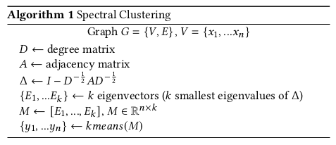
Now that we have looked at the use of Laplacian eigenvectors as positional encoders, let’s see how informative these eigenvectors are to the structure and connectivity of the graph. A short mathematical overview of why these recapitulate a graph’s connectivity can be found at appendix A. To validate this empirically, we performed a simple experiment making sole use of the Laplacian eigenvectors to try and perform node classification via spectral clustering. Spectral clustering on the graph (see Algorithm 1 for description of the method) allows us to perform unsupervised clustering of the nodes into a predefined number of classes. We rearranged the clusters’ names by using a hungarian algorithm, to fall back on the labels from the node classification task, which enabled a comparison of node classification performance using only these eigenvectors compared with the full Graph Transformer architecture.

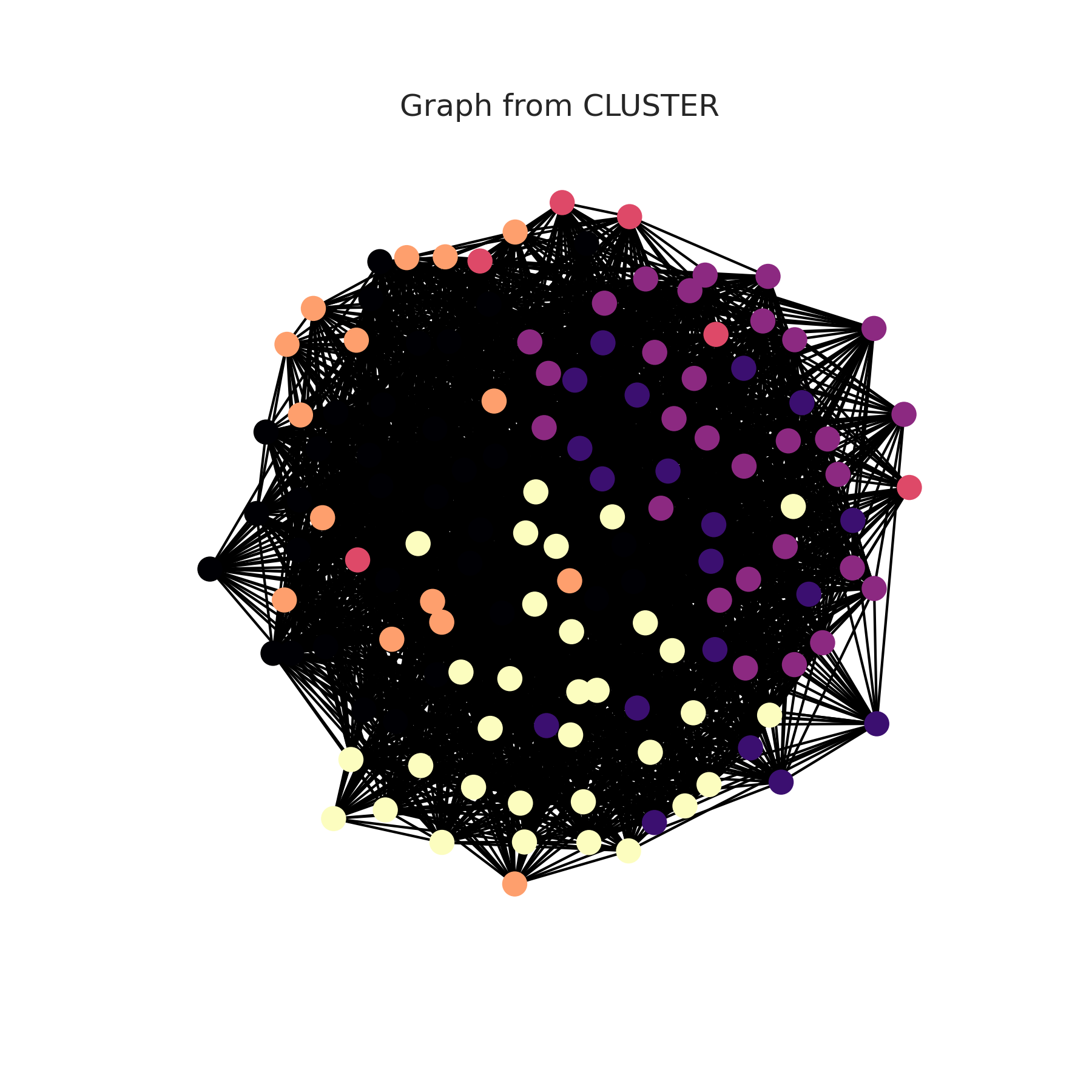
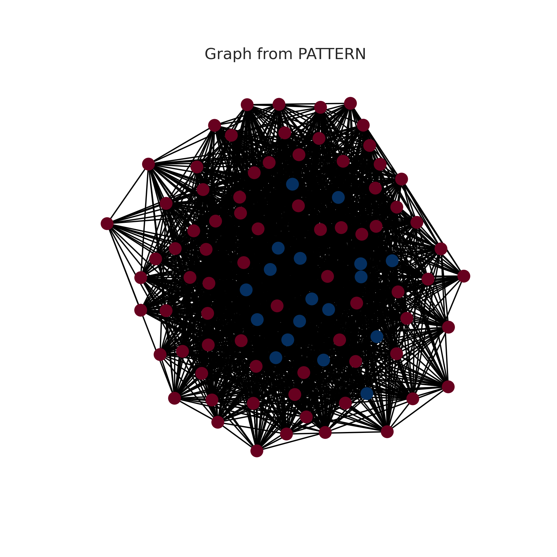
We tested our experiment on CLUSTER and PATTERN’s datasets, which led to the results presented in Figure 3. We obtained far better results than random on the CLUSTER dataset, in which nodes are classified in six classes, however we did not outperform a random classification on the PATTERN dataset, in which nodes are classified only in two classes, which makes it easier for a random classification to perform correctly. Overall this still shows that the Laplacian eigenvectors provide structural information that can help with a node classification task if the underlying graph structure means that highly connected nodes also tend to have similar class labels, which seems to be the case on the CLUSTER dataset. But as shown by the large performance difference with GT, positionnal encodings cannot be used alone if we want to have good results.

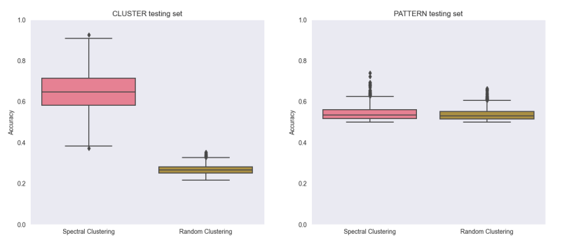
We obtained far better results than random on the CLUSTER dataset, in which nodes are classified in six classes, however we did not outperform a random classification on the PATTERN dataset, in which nodes are classified only in two classes, which makes it easier for a random classification to perform correctly. Overall this still shows that the Laplacian eigenvectors provide structural information that can help with a node classification task if the underlying graph structure means that highly connected nodes also tend to have similar class labels, which seems to be the case on the CLUSTER dataset. But as shown by the large performance difference with GT, positionnal encodings cannot be used alone if we want to have good results.

Performance of other algorithms on these datasets

Other methods that are simpler than graph neural networks can also be used as simpler benchmarks when looking at the graph prediction tasks. We therefore chose to perform graph regression on the ZINC dataset (subset) thanks to a graph kernel method, wanting to quantify the performance of a non neural-network based algorithm. The kernel function allows us to compute similarities between pairs of graphs, by calculating an inner product of two graphs.

We chose to use the Weisfeiler Lehman kernel (Shervashidze, 2011), which works as follows :

• Compute a sequence of $h$ Weisfeiler Lehman graphs, thanks to the Weisfeiler Lehman isomorphism test \(G_1, ...., G_h\) and \(G_1', ... G_h'\) for two graphs \(G\) and \(G'\)
• Compute the weisfeiler lehman kernel \(w_{kl}(G, G') = k(G_1, G_1') + ... + k(G_h, G_h')\) where \(k\) can be any graph kernel. The simplest one would be \(k = <hist_G, hist_{G'}>\) where \(hist_G\) is the histogram of vertex labels, meaning the frequencies of compressed labels. The Weisfeiler Lehman algorithm proceeds as follows :

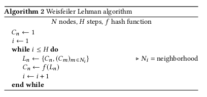
\(C_n\) can be interpreted as a compressed label of node \(n\), whereas \(L_n\) is a multi-set of compressed labels of each neighboring node. The hash function \(f\) should output a unique value for each representation, and can be chosen arbitrarily. Figure 5 shows a graphical illustration of this algorithm. Values taken by $f$ are chosen random for the sake of the example.

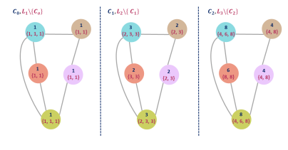
We obtained a MAE of \(0.48\), which is a poor result compared to the ones given by other methods : \(0.276\) for GT, \(0.214\) for Gated GCN, \(0.384\) for GAT, and \(0.367\) for GCN. This confirms the need for perhaps more complex methods to obtain better performance.

Generalizability and reproducibility

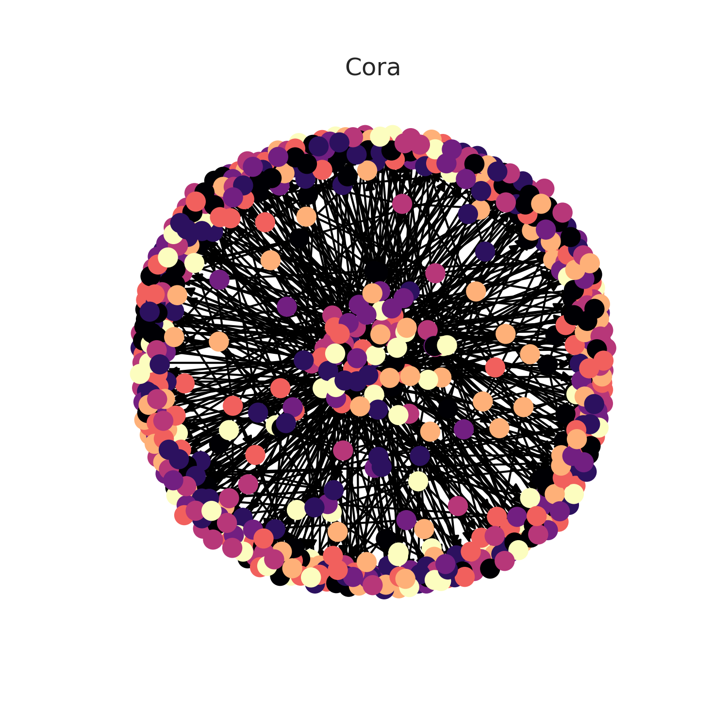
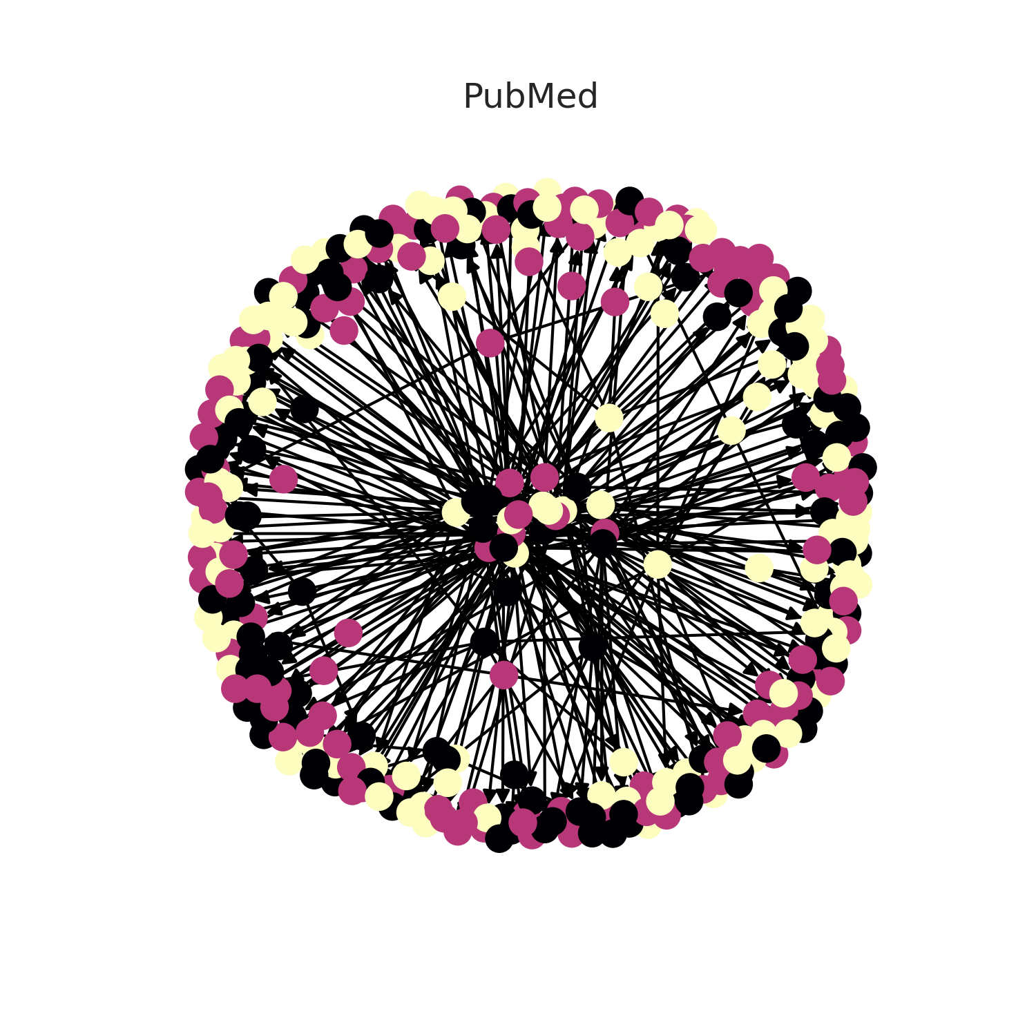
To have an in-depth look at the original code, we decided to run graph transformers on another dataset that was not present in the original paper or in the benchmarking-gnns repository that is maintained by the same authors . We chose the Pubmed and Cora (Sen et al., 2008) node classification benchmarks as they are some of the most highly used node classification benchmarks in the graph machine-learning field with hundreds of papers citing each one per year with results available on papers with code. Although the overall results of the paper were reproducible, the code was very difficult to apply to the Pubmed dataset. No real packaging effort made the code’s adaptability very limited. No instructions are provided to run on other datasets, and no real overview of the repository structure is provided. To run the graph transformers architecture on Pubmed, we had to (i) create a custom dataset class to load the pytorch geometric dataset in the very specific format required by the training scripts (ii) rewrite the main training and data loading scripts to run graph transformers as many lines of code were dataset specific (iii) correct some minor parts of the actual architecture. The custom dataset class involved making the original pytorch geometric dataset compatible with the Deep Graph Library (dgl). However, the original code made use of several intermediate dataset classes before the final one obscuring the preparatory steps needed. Overall, the changes made are available on the project github.

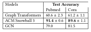
As we can see, the performance on these other datasets is quite poor when compared to the state-of-the-art methods. It should be noted that out-of-the-box hyperparameters were chosen with little additional tuning meaning the results could probably be improved by spending more time fine tuning parameters. The results provided were calculated over 3 runs for GT and the others were obtained from open benchmark results.

Conclusion

In conclusion, graph transformers are an interesting proof of concept of how the transformer architecture may be adapted to work on homogeneous graphs with arbitrary structure for various prediction problems. Although they do not beat the state-of-the-art as of yet, they present a promising avenue for further research in the area as transformers have showcased impressive performance in lots of adjacent domains. The key insights to adapt the transformer to graphs is the use of laplacian eigenvectors for positional encoding, the use of graph sparsity as in inductive bias in the node updates and the inclusion of edge features in the attention calculation. Much theoretical work remains to correctly analyze the full expressivity of graph transformers for graph prediction problems, build on the proposed proof of concept to actually obtain competitive results and make it a usable architecture by integrating it into popular online model repositories and working on the code’s cleanliness.

References

1. A Generalization of Transformer Networks to Graphs

   Dwivedi, Vijay Prakash, and Bresson, Xavier

   2020
2. Representation Learning on Graphs: Methods and Applications

   Hamilton, William L., Ying, Rex, and Leskovec, Jure

   2017
3. Node Classification in Social Networks

   Bhagat, Smriti, Cormode, Graham, and Muthukrishnan, S.

   2011
4. Graph Kernels

   Vishwanathan, S. V. N., Borgwardt, Karsten M., Kondor, Imre Risi, and Schraudolph, Nicol N.

   2008
5. Laplacian Eigenmaps and Spectral Techniques for Embedding and Clustering

   Belkin, Mikhail, and Niyogi, Partha

   In Proceedings of the 14th International Conference on Neural Information Processing Systems: Natural and Synthetic 2001
6. node2vec: Scalable Feature Learning for Networks

   Grover, Aditya, and Leskovec, Jure

   In Proceedings of the 22nd ACM SIGKDD International Conference on Knowledge Discovery and Data Mining 2016
7. The Graph Neural Network Model

   Scarselli, Franco, Gori, Marco, Tsoi, Ah Chung, Hagenbuchner, Markus, and Monfardini, Gabriele

   IEEE Transactions on Neural Networks 2009
8. Geometric Deep Learning: Going beyond Euclidean data

   Bronstein, Michael M., Bruna, Joan, LeCun, Yann, Szlam, Arthur, and Vandergheynst, Pierre

   IEEE Signal Processing Magazine 2017
9. Attention Is All You Need

   Vaswani, Ashish, Shazeer, Noam, Parmar, Niki, Uszkoreit, Jakob, Jones, Llion, Gomez, Aidan N., Kaiser, Lukasz, and Polosukhin, Illia

   2017
10. Graph-Bert: Only Attention is Needed for Learning Graph Representations

    Zhang, Jiawei, Zhang, Haopeng, Xia, Congying, and Sun, Li

    2020
11. Benchmarking Graph Neural Networks

    Dwivedi, Vijay Prakash, Joshi, Chaitanya K., Luu, Anh Tuan, Laurent, Thomas, Bengio, Yoshua, and Bresson, Xavier

    2020
12. Convergence of Laplacian Eigenmaps

    Belkin, Mikhail, and Niyogi, Partha

    In Advances in Neural Information Processing Systems 2006
13. Weisfeiler-lehman graph kernels

    Shervashidze, Nino

    Journal of Machine Learning Research 2011
14. Collective Classification in Network Data

    Sen, Prithviraj, Namata, Galileo Mark, Bilgic, Mustafa, Getoor, Lise, Gallagher, Brian, and Eliassi-Rad, Tina

    AI Magazine 2008

Appendix

A - Laplacian eigenvectors

We consider here the non-normalized graph Laplacian matrix (which is positive semi-definite) defined as \(L = D-A\) with \(D\) the degree matrix and \(A\) the adjacency matrix as defined in the beginning of the paper. We first note that the vector \(x_0 = (1, ..., 1)\) is an eigenvector associated to the eigenvalue 0. This is simply the result of the properties of \(D\) and \(A\) since \(D_{ii} = \sum\limits_{j=1}^{N}A_{ij}\). The second smallest eigenvalue can be found by solving the optimization problem: \(\min_{\|x\|=1, x\perp x_0} x^TLx\) The term we optimize can be rewritten as \(x^TLx = \sum\limits_{i=1}^{N}\sum\limits_{j=1}^{N}x_i(D_{ij} - A_{ij})x_j\) \(=\sum\limits_{i=1}^{N}x_i^2D_{ii} - \sum\limits_{i=1}^{N}\sum\limits_{j=1}^{N}x_iA_{ij}x_j\) \(=\sum\limits_{(i, j)\in E}x_i^2 + x_j^2 - 2\sum\limits_{(i, j)\in E}x_ix_j\) \(=\sum\limits_{(i, j)\in E} (x_i - x_j)^2\) The final equation shows that nodes that are connected (in E) will have similar values when looking at the eigenvector associated to the smallest eigenvalues. Therefore, taking the eigenvectors associated with the smallest eigenvalues gives an indication of connectivity since nodes with similar values across the k smallest eigenvectors will tend to be highly connected.